Exploring the Home Mortgage Market using Spark on Google Cloud

Overview

In this comprehensive analysis, we delve into the intricate dynamics of the US Home Mortgage market. Utilizing an extensive dataset released under the Home Mortgage Disclosure Act (HMDA)Enacted by Congress in 1975 to provide public loan data that can be used to assist in determining whether financial institutions are serving the housing needs of their communities., we aim to uncover patterns and correlations across various dimensions such as gender, race, income, property type, loan type, amount, and geographical location.

Our insights are geared towards enabling financial institutions to enhance their decision-making, while exposing biases that still exist in the modern lending landscape.

The Dataset: A Data Engineer's Dream (and Nightmare)

Our analysis leverages a detailed dataset encompassing Mortgage applications specifically for first lien, owner-occupied, 1-4 family homes, collected under the HMDA regulations for the years 2016 and 2017.

It includes crucial data points on loan attributes, property specifics, applicant demographics, and lender details, all while maintaining stringent privacy standards for applicants and borrowers. This invaluable dataset has been sourced directly from the Consumer Financial Protection Bureau (CFPB)A U.S. government agency that makes sure banks, lenders, and other financial companies treat you fairly..

Insightful Findings: What the Data Tells Us

Our meticulous analysis of over 13 million mortgage applications utilizing PySpark on Google Cloud Dataproc revealed several key disparities and trends:

• Gender Bias: The dataset shows a noticeable skew towards male applicants, highlighting a persistent gender disparity in the mortgage market.
• Race and Income Correlation: A clear correlation exists between an applicant's race and their income levels, with consequential effects on loan amounts.
• Loan Amount Discrepancies: A significant gap is evident in the average loan amounts sought by Asians and Whites compared to other racial groups, a gap which actually increases with income.
• Geographical Variations: Debt-to-income ratios exhibited stark differences across states. Unsurprisingly, Californians showed vastly higher ratios compared to Midwestern and Eastern states.

Deep Dive: Data Exploration & Visualizations

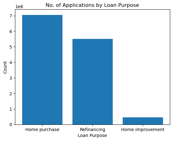
1. Distribution of Loans by Purpose

A significant discovery was the predominance of home purchases as the top loan purpose, totaling around 7 million applications. This is followed by refinancing and home improvement loans.

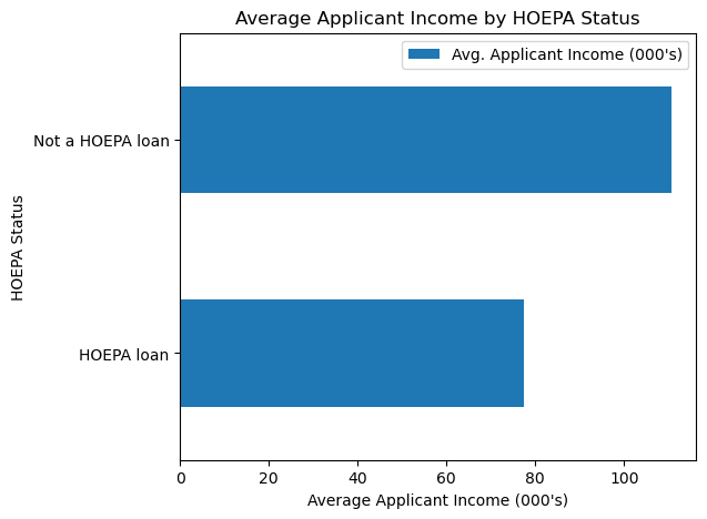
2. Income of HOEPA vs Non-HOEPA Applicants

When dissecting the data by HOEPA statusThe Home Ownership and Equity Protection Act (HOEPA) was enacted in 1994 to address abusive practices in refinances and closed-end home equity loans with high interest rates or high fees., we observed a notable difference. Non-HOEPA loan applicants displayed higher average incomes (over $100k), while HOEPA loans stayed below$80k.

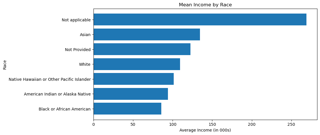
3. Mean Income by Race

An analysis of mean income by race presented significant, uncomfortable disparities. Keeping aside the Not applicable categories, Asian Americans have the highest mean income of $135,000 per year</span>, followed by Whites at$105,000 per year. Native Americans, Black or African Americans, and Native Hawaiians earn less than $100,000 per year on average.

4. Average Debt-to-Income Ratio by State

The Debt-to-income ratio graph reveals that states on the west coast, particularly California, have substantially higher ratios than states on the east coast. This means the loan amount Californians apply for is relatively higher compared to their actual income.

Predictive Analysis using PySpark MLlib

We didn't just want to look at historical data; we wanted to predict it.

Data Preparation

First, we had to address the massive skew in income (highly right-skewed). We utilized the Interquartile Range (IQR) method with a multiplier of 1.5 to remove extreme outliers in both Income and Loan Amount to normalize our training data.

We then divided columns into categorical and continuous groups:

# Detect categorical and numerical columns dynamically
categorical_columns = [field[0] for field in data_correct_type.dtypes if field[1] == "string" and field[0] != 'loan_amount_000s']
continuous_columns = [field[0] for field in data_correct_type.dtypes if field[1] != "string" and data_correct_type.select(field[0]).distinct().count() > 20 and field[0] != 'loan_amount_000s']

Building the ML Pipeline

We indexed, One-Hot Encoded, and assembled the features before scaling them:

# Index and one-hot encode categorical columns
indexers = [StringIndexer(inputCol=col, outputCol=f"{col}_index", handleInvalid="skip") for col in categorical_columns]
encoders = [OneHotEncoder(inputCol=f"{col}_index", outputCol=f"{col}_ohe") for col in categorical_columns]

# Assemble and Scale
assembler = VectorAssembler(inputCols=[f"{c}_ohe" for c in categorical_columns] + continuous_columns, outputCol="features")
scaler = StandardScaler(inputCol="features", outputCol="scaledFeatures")

# Train the model
model = LinearRegression(featuresCol='scaledFeatures', labelCol='loan_amount_000s', maxIter=10, regParam=0.3, elasticNetParam=1)
pipeline = Pipeline(stages=indexers + encoders + [assembler, scaler, model])

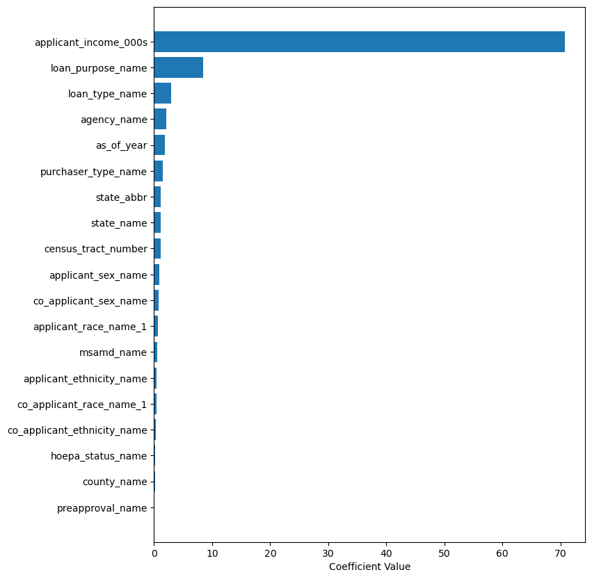
Results & Feature Importance

After evaluating the model (RMSE: 82.90), we backtracked the coefficients to find the most relevant columns determining Loan Amount:

1. Applicant Income: Directly corresponds to borrowing capacity.
2. State Name: Dictates real estate baseline pricing.
3. Loan Purpose / Type: Home purchases involve much larger sums than home improvement.

Conclusion and Next Steps

The U.S. home mortgage market is highly diverse. While our model showed race and gender didn't heavily weight the amount of the loan linearly, the exploratory data clearly shows massive disparities in who is applying and their baseline incomes.

Pertaining to the Regression section, we observed that the plot for Predicted vs. Actual values was slightly skewed, indicating the relationship between Income and Loan Amount may not be strictly linear.

Next Steps: We plan to explore using Polynomial Expansions of the Income feature to better fit the regression model, or perhaps pivot to a Gradient Boosted Tree (GBTRegressor) to capture non-linearities automatically!